This week we’re connecting our boards to “the outside world” (by which I mean, to take it out of the Arduino IDE) and create an interface for it! I decided that I wanted to visualize just one number, the value from the phototransistor from my very first board, in somewhat silly ways, using several of the most common tools to visualize data on the web; D3.js + SVG, HTML5 canvas, WebGL + Three.js & p5.js.
Assignments
Our tasks for this week are:
- Group assignment: Compare as many tool options as possible
- Individual assignment: Write an application that interfaces a user with an input &/or output device that you made
Hero Shots
Showing some final results of the “silly” visualizations of one number that I created with D3.js, SVG, HTML5 canvas, Three.js, and p5.js for the tl;dr and hopefully showing you why the rest of this very long blog could be interesting to read (⌐■_■)


Programming a Board
I wrote a really simple program that uses the phototransistor on the very first “Hello World” board that I made during the “Electronics Design” week. It merely reads the analog value and uses a Serial.println to send it out:
#define PIN_PHOTO 1 //ATtiny412 PA7

void setup() {
  // Initialize serial communication
  Serial.swap(1); //use alternate TX/RX positions
  Serial.begin(9600);
  while(!Serial);

  pinMode(PIN_PHOTO, INPUT);
}//void setup

void loop() {
  int sensor_value = analogRead(PIN_PHOTO);
  Serial.println(sensor_value);

  //byte mapped_value = map(sensor_value, 0, 1023, 0, 255);
  //Serial.write(mapped_value);

  delay(100);
}//void loop
I also tried using Serial.write() a few times, but I could never get it to result in useful data coming into the serial ports on the other side.
Serial on the Web
To be able to access the results that are returned by my board through the UART (TX and RX) of the FTDI and USB into a different program, we’ll need a serial port. As with anything on the web, there are undoubtedly several ways of doing it.
SerialPort Package
The first one I came across was the SerialPort package, which is a Node.js package.
I already have Node and npm (Node’s package manager) installed because I use it for my work somewhat often, although I’m by no means an expert.
I started by following the installation instructions. I created a new folder in my localhost, set-up a new node project with npm init, which gives you a package.json file, and installed the SerialPort package with npm install serialport.
Following the usage page, I tried to write the most simple code snippet that receives the data from my board and prints it to the terminal.
Although Node.js uses JavaScript, it’s actually run outside of a browser. So in order to run a script written with Node.js packages (easily) you run node index.js in the terminal, where index.js is the script that you want to run.
I had a connection set up pretty quickly, but the results returned looks like <Buffer a7>. Searching a bit further and I saw that I had to add a parser to “decode” the incoming data. Another code example later and I had the data coming into my terminal:
//Set up the port
const SerialPort = require('serialport')
const port = new SerialPort('/dev/tty.usbserial-D30A3T7C', {
    baudRate: 9600
})

//Create a parser to read the incoming data
const ReadLine = require('@serialport/parser-readline')
const parser = new ReadLine({delimiter: '\r\n'});

//Attach the parser to the incoming data
port.pipe(parser);

//Run the "readSerialData" function on every new stream of data
parser.on('data', readSerialData);

function readSerialData(data) {
    console.log(data);
}//function
I could cover up the phototransistor and see the numbers rise to ~800:
Note | You can stop a Node.js script (that keeps going) in the terminal by typing CTRL+C.
Connecting to a Browser
I now had the data being output in my terminal. I searched online for a way to get this straight into a browser. I found that socket.io would be a good match for the SerialPort package. On their page is an example that shows how to create a chat application. It wasn’t quite what I needed, but the snippet of code under the Integrating Socket.IO header was useful because it shows how to set-up a web server with the express and http packages, and how to integrate socket.io into that. I installed all of these with npm install.
I did run into an error when I started the webserver and loaded the localhost on my browser that it couldn’t find any file other than the index.html. Thankfully, I found that you can add app.use(express.static(path.join(__dirname, '/'))); to the code to fix this.
Combining the example on the socket.io website, and this stackOverflow question I managed to get it all working, and have the phototransistor value from my board be displayed in the browser.
I have a server.js file that contains the calls to create the web server, to open the socket on the server-side, and to use the serial port code I figured out before:
/////// Express & Socket.io ///////
const path = require('path');
const express = require('express');
const app = express();
const http = require('http');
const server = http.createServer(app);
const port_num = 3000;

const { Server } = require("socket.io");
const io = new Server(server);

//Had to add this otherwise it wouldn't work
app.use(express.static(path.join(__dirname, '/')));

app.get('/', (req, res) => {
    res.sendFile(__dirname + '/index.html');
})

io.on('connection', (socket) => {
    console.log('a connection found');
    socket.on('disconnect', function(){
      console.log('disconnected');
    });
})//io.on

server.listen(port_num, () => {
    console.log(`listening on *:${port_num}`);
})

/////// Serial port ///////
const SerialPort = require('serialport');
const port = new SerialPort('/dev/tty.usbserial-D30A3T7C', {
    baudRate: 9600
})
const ReadLine = require('@serialport/parser-readline')
const parser = new ReadLine({delimiter: '\r\n'});

port.pipe(parser);
parser.on('data', readSerialData);

function readSerialData(data) {
    console.log(data);
    io.emit('parsed-data', data);
}//function readSerialData
Then there is a simple index.html:
<!DOCTYPE html>
    <head>
        <meta charset="utf-8">
        <title>JavaScript | Fab Academy</title>
        <meta name="author" content="Nadieh Bremer">

        <!-- JavaScript files -->
        <script src="/socket.io/socket.io.js"></script>
    </head>
    <body>
        <h3 id="text-value">X</h3>

        <!-- Custom JavaScript -->
        <script src="script.js"></script>
    </body>
</html>
And finally, there is a script.js that gets called within the index.html. This gets the parsed serial data and uses it to update a text value (this is called the client side, whereas the server.js script is called server side):
let socket = io();

let dataDisplay = document.getElementById("text-value");

socket.on('connect', function () {
  socket.on('parsed-data', function (data) {
    //console.log(data);
    dataDisplay.innerHTML = data;
  })
})//socket.on
I then run node server.js in my terminal, and go to http://localhost:3000/ to see the result of the phototransistor in the browser:
Now that I had the data coming into the browser, I could experiment with different browser-based packages/ways to visualize that one incoming number.
Usually I visualize hundreds to millions of data points, so visualizing just one number, the value from the phototransistor, felt somewhat new. I wanted to explore a few different ways to tackle it; using the strengths of each specific tool.
D3.js & SVG
In my day-to-day work I’m a freelancing data visualization designer. I create static and interactive visuals meant for print and online. One of the “tools” I use almost daily in my work is D3.js. It has basically become the standard in online data visualization.
It’s not easy to learn though. When I was completely new to the web, it took me a whole week to create a scatterplot with D3.js that had some simple hover animation going on. I like the following way that D3.js has been described to me: “D3 makes easy things hard, and hard things easy”. In essence, D3 gives you access to many low-level functions, which makes it hard to create a “simple” line chart. However, once you’ve crossed that hurdle, and understand how D3.js works, those low-level functions give you an amazing amount of freedom to use and combine them in different ways to make data visual in ways that click-and-drag tools just can’t do.
Most of the work in my portfolio has incorporated D3.js. Not always to do the actual drawing, but always to prepare things, such as hierarchies, scales and colors.
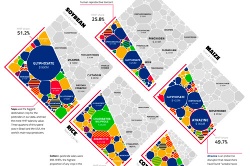
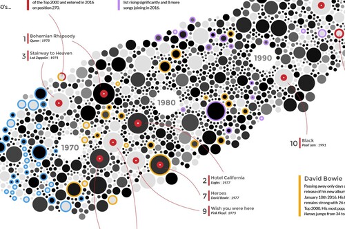
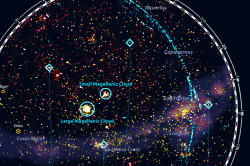
Below are a few sneak peeks from some of my works where D3.js played a big role and I visualized the results using SVGs; Highly Hazerdous Pesticides for Unearthed the journalistic arm of Greenpeace, Space Wars for Scientific American, a personal project about the Top 2000 songs, and Digital Trackers for the New York Times.
![]()
The “heart” of D3.js is the enter-update-exit flow. It is the way to turn SVG elements into a data visualization that can either be static or update with real-time data. I therefore wanted to incorporate a typical enter-update-exit into this visual. Plus, I wanted to do it using SVGs. Although D3.js has many functions that can work well with HTML5 canvas these days, it started out with an aim at SVGs.
My idea was to recreate the feeling of those old equalizer bars that were often used to visualize the volume of music; using one “stack” of small rectangles whose height would be determined by the value returned by the phototransistor.
I downloaded the d3.zip file, and placed the d3.min.js file into a (new) lib folder within my project folder. Within the index.html I added <script src="lib/d3.min.js"></script> to the head. I also added a div to the body with <div id="chart"></div> to which I could append the visualization.
Within the script.js I added some code to create an SVG:
//Create SVG
const width = 500
const height = 850

//Append an SVG to the div with id "chart"
const svg = d3.select("#chart").append("svg")
    .attr("width", width)
    .attr("height", height)
    .attr("class", "svg-chart")
As a simple start I added a rectangle across the full background, and a text right in the center, both of which would update in color depending on the value. First just from white to black (or vice versa for the text), using a d3.scaleLinear():
//Color scale to go from black to white between the values 500 - 950
const scale_color_bw = d3.scaleLinear()
    .domain([500, 950])
    .range(["black", "white"])
    .clamp(true)

///////////////////// Background color ////////////////////
const rect_background = svg.append("rect")
    .attr("class", "background")
    .attr("x", 0)
    .attr("y", 0)
    .attr("width", width)
    .attr("height", height)
    .style("opacity", 0.7)

function updateBackground(data) {
    rect_background.style("fill", scale_color_bw(data))
}//function updateBackground

////////////////// Text on the background /////////////////
const text_value = svg.append("text")
    .attr("class", "background-text")
    .attr("transform", `translate(${width/2}, ${height/2})`)
    .style("text-anchor", "middle")
    .style("font-size", "170px")

function updateText(data) {
    text_value
        .style("fill", scale_color_wb(data))
        .text(data)
}//function updateText
I added the two update functions (updateBackground(data); updateText(data);) to the inner socket.on function, so they’d be called whenever the socket received a new value.
For the central bar chart I created a group (g in SVG) to which the small rectangles could be appended. I then used D3’s enter-update-exit flow to check at each time:
- How many bars are there already
- How many bars should be drawn based on the new data
- If fewer bars should be draw, which should be removed, and remove those
- If more bars should be drawn, draw them
The code below essentially only does the exit and enter part, because no update of existing bars is needed:
//////////////////////// Bar chart ////////////////////////
const bar_group = svg.append("g")
    .attr("class", "bar-group")
    .attr("transform", `translate(${width/2}, ${0})`)

const bar_width = 25
const bar_height = 6

function updateBars(data) {
    let num_bars = Math.round(data/10)

    //Append new data to the group
    let bars = bar_group.selectAll(".bar")
        .data(d3.range(num_bars), d => d)

    //EXIT
    bars.exit().remove()

    //ENTER
    let enter_bars = bars.enter()
        .append("rect")
        .attr("class", "bar")
        .attr("id", d => `bar-${d}`)
        .attr("x", -bar_width/2)
        .attr("y", d => height - d * (bar_height + 2))
        .attr("width", bar_width)
        .attr("height", bar_height)
        .attr("rx", bar_height/2)
        .style("fill", d => scale_color_bars(d * 10))
}//function updateBars
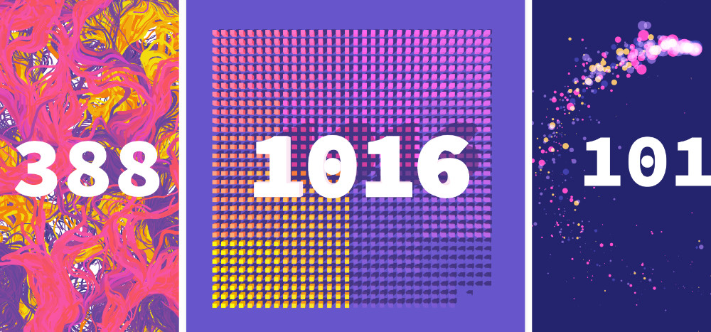
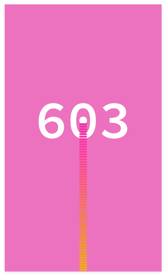
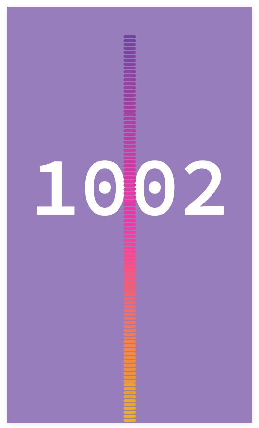
I felt that the black-white was a bit too boring, so I added a splash of color and ended up with the following result:
Below are three snapshots; from shining a flashlight on the phototransistor, resulting in really low values, to the average light levels in my room (while it was sunny), to covering up the phototransistor in the right-most image:
Below you can find the full folder with all the JavaScript and HTML files required to run the above example. I’ve removed the node_modules folder because it’s insanely big, and you can install the required node modules by running npm install (without any dependencies) in the terminal when you’re in the folder.
- D3.js+SVG-based visual files | ZIP file
HTML5 Canvas
I find HTML5 Canvas to be quite straightforward. It’s easy to implement something simple, the code speaks for itself. Only when you’re looking into animations and interactions do things get harder than doing it with SVGs. A benefit of canvas is that it performs much better than using SVGs, because the browser needs to keep a tab on all SVG elements, but there’s only one PNG that you’re creating with canvas. You can see the difference a little as follows: SVG is like Adobe Illustrator while canvas is like Adobe Photoshop.
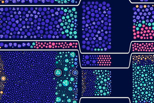
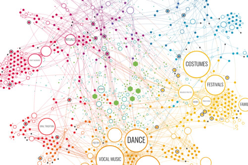
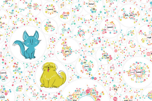
Below are a few sneak peeks at a selection of my works where visualizing the results with canvas played a big role; Re-imagining the Golden Record for Sony Music Entertainment, Hubble’s 30-year legacy for Physics Today, Dive into your Cultural Heritage for UNESCO, and Why do cats and dogs for the Google.

Besides how straightforward its code is, and how well it performs, another reason why I like working with HTML5 canvas is that it’s native to the web. There’s no need to load any external library, such as I had to do with D3.js.
I wanted to create something with canvas that could not have worked with SVG due to performance reasons. However, how do you create hundreds of “elements” when all I’m getting is one number. That’s when I remembered something that I made years ago using exploding particles (which in itself was heavily based on a demo).
I wanted to have a ring of exploding particles moving around and around, where the speed of movement and the number of particles being “ejected” were determined by the phototransistor value.
With a new script.js I created the canvas and context variables, the latter of which is what you use to draw on.
To take the fact into account that canvas will look blurry on retina device I’m using a “crispy-canvas” approach where I’m making a canvas that’s twice as big in width and height, and then scaling it all down to the original width and height:
/////////////////// Set-up the Container //////////////////
//Set-up the canvas
const canvas = document.createElement("canvas")
const ctx = canvas.getContext("2d")

//Update the canvas size - taking retina devices into account
const pixel_ratio = 2 //for retina devices
canvas.width = width * pixel_ratio
canvas.height = height * pixel_ratio
canvas.style.width = `${width}px`
canvas.style.height = `${height}px`
ctx.scale(pixel_ratio, pixel_ratio)

//Move the origin to the center
//This is easier when working with a circular layout
ctx.translate(width/2, height/2)

//Add the canvas to the "chart" div
document.getElementById("chart").appendChild(canvas)
To show a font on a canvas it needs to be loaded first. Since I have nothing else in my HTML in terms of text I’m using the document.fonts.load function. If I was to be very specific I’d also use the documents.fonts.ready.then() function to check when the font is loaded. However, in this case the visual gets updated several times a second anyway, so I don’t mind if the first few frames are with the default font.
After the font is loaded I set its style with the .font, .textBaseline, and .textAlign options. Because I’m always drawing the same style of text, I only need to set this once, and thus only have the call to the color, .fillStyle, and the drawing of the text within the updateText() function:
//Load the font for usage in the canvas
const font_name = 'Source Code Pro'
document.fonts.load(`normal 900 10px "${font_name}"`)

////////////////// Text on the background /////////////////
//Set the font - only once, since we're never changing it
ctx.font = `900 normal 180px ${font_name}`
ctx.textBaseline = "middle"
ctx.textAlign = "center"

function updateText(data) {
    ctx.fillStyle = scale_color_bw(data)
    ctx.fillText(data, 0, 0)
}//function updateText
Like before, add the updateText() function to the socket function to have it run every time a new serial value comes in.
One extra thing needs to be added, because canvas is transparent by default. Thus if I were to run the above code, I’d see text being overplotted on itself. I therefore fill the canvas with a white rectangle before every call to updateText():
ctx.fillStyle = "white"
ctx.fillRect(-width/2, -height/2, width, height)
This could’ve also been done with .clearRect(), but I want to play with the background color later.
I then started adding the “particles”. Using the code I already had from my original example it didn’t take long to go from simple static circles to total chaos:
The latter of which is better shown as a video:
Which was merely an issue of setting the blending mode of the canvas to multiply for the circles (so they look good when overlapping), but not setting it back to the default source-over when drawing the white background rectangle. Adding ctx.globalCompositeOperation = "source-over" above the background rectangle code fixed the issue.
However, I felt that the result looked quite jagged, not a smooth animation:
I realized that having set a delay(100) within the Arduino code, meant that the canvas was only updated 10x a second, which is too slow for smooth animation in our eyes. I therefore had to decouple the number of times that the canvas was drawn from the time when data came in from the serial port (I also could’ve removed the delay() from my board, but I wanted to use the same base code for all my visuals).
For this I took the code to update the visual from the socket.on function and put it its own function:
function draw() {
    if(serial_data) { //Only draw if serial_data is known
        //Update the background
        ctx.globalCompositeOperation = "source-over"
        ctx.fillStyle = "white"
        ctx.fillRect(-width/2, -height/2, width, height)

        updateText(serial_data)
        updateParticle(serial_data)
    }//if
    requestAnimationFrame(draw)
}//function draw
draw() //call for the first time
At first I used requestAnimationFrame(), which calls the draw function again when the browser is ready. It’s a really handy function. However, when I reloaded the page, it was all going much too fast!
In those cases I simply create an interval with setInterval(draw, 20), which calls the draw function every 20 milliseconds (and removed the requestAnimationFrame(draw) line from the draw function). An interval of 20 milliseconds gave a good result in terms of speed.
I added several more visual tweaks, such as using the same color palette as for the SVG visual, moving around a smaller radius for lower values, and even bigger text. The final result looks as follows, where I’m either moving in my flashlight over the phototransistor (low values), or covering the phototransistor (high values):
Below you can find the full folder with all the JavaScript and HTML files required to run the above example. As before, I’ve removed the node_modules folder because it’s insanely big, and you can install the required node modules by running npm install (without any dependencies) in the terminal when you’re in the folder.
- HTML5 canvas visual files | ZIP file
WebGL & Three.js
Three.js is a wrapper that makes it much much easier to work with WebGL. I personally see WebGL as the way to go if I need to visualize an insane number of datapoints, where even canvas can’t handle it anymore, and I need to power of visualizing with the GPU instead of the CPU. My other reason to go for WebGL is to make something in 3D. However, generally 3D is not a good option for data visualization.
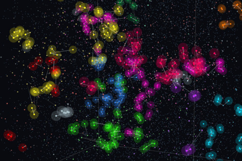
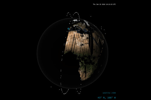
Because I don’t often have an insane amount of (moving) data to visualize, nor need to make things in 3D, I don’t have that much experience with WebGL or Three.js. Below are two of my few WebGL projects. For the left I used Three.js for its 3D capabilities to visualize a simulation about alien colonization, while for the right it was primarily because I had to loop through a dataset of 600,000 rows and draw them as fast as possible to visualize how satellites are taking a full image of the Earth every day (this was actually made with regl, not Three.js)
With Three.js I wanted to create something that I couldn’t have done with either SVGs or HTML5 canvas. At first I was thinking of moving through a 3D environment as a rollercoaster, where the direction and environment would change depending on the value returned by the phototransistor.
However, once I started investigating this idea more, I realized that it was too much for my knowledge right now, and the amount of time I’d given myself to work on this (±3 hours).
I then thought it might be interesting to recreate that SVG example, but do it in 3D instead, applying shadows and being able to move around the scene.
I went the the installation page of Three.js. Interestingly, the only way to load Three.js is through a module (the way Node.js works), even directly in the browser. You have to add type="module" to the script tag. I wasn’t aware that this was now truly supported.
It’s been at least six months since the last time I worked with Three.js, so I started with the basic example from the Three.js page to create a simple rectangle:
import * as THREE from 'https://cdn.skypack.dev/three@0.128.0'

///////////////// Setup the Three.js scene ////////////////

//Create the Three.js scene
const scene = new THREE.Scene()

//Setup the canvas and webGL renderer and add it to the HTML
const renderer = new THREE.WebGLRenderer({ antialias: true})
renderer.setSize( width, height )
container.appendChild( renderer.domElement )

///////////////////// Setup the camera ////////////////////

//Set up a camera for the viewer to see into the scene
//Field-of-view, aspect ratio, near & far clipping place
const camera = new THREE.PerspectiveCamera( 75, 1, 0.1, 1000 )
camera.position.set(0, 0, 5)

///////////////////// Add Cube ////////////////////
const geometry = new THREE.BoxGeometry()
const material = new THREE.MeshBasicMaterial( { color: "#10a4c0" } )
const cube = new THREE.Mesh( geometry, material )
scene.add( cube )

///////////////////////// Animate /////////////////////////
function animate() {
    //Update scene
    renderer.render( scene, camera )
    requestAnimationFrame( animate )
}//function animate
animate()

Next, I added a ground plane with new THREE.PlaneGeometry to act as a floor for the cube.
I also added lights so I could show shadows from the cube on the plane and drive home the 3D element. I generally add a soft THREE.AmbientLight which lights the scene equally and doesn’t cast shadows. Next, I added a THREE.DirectionalLight, which acts as a light that shines from one direction, seemingly coming from infinitely far away, like the Sun.
//Ambient light
const light = new THREE.AmbientLight( "#fbe7f2", 1 )
scene.add( light )

//Directional light
const light_direction = new THREE.DirectionalLight("#ffffff", 0.8)
light_direction.castShadow = true
light_direction.position.set(-20, -15, 20)
light_direction.target.position.set(0, 0, 0)
//Add directional light and its target to the scene
scene.add(light_direction)
scene.add(light_direction.target)

//Show helper to show direction and location of light
const helper = new THREE.DirectionalLightHelper(light_direction)
scene.add(helper)
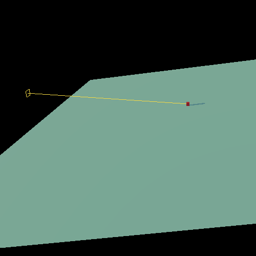
The light helper is a very useful way to see the point where you’ve placed the light and in which direction it’s pointed. In the two images below the yellow line is from the helper, pointing towards the center of the scene.
To make the shadows actually appear, I need to set this to the light, both the cube and the plane, but also activate shadows in general. They’re computationally expensive to calculate and are thus not activated by default.
//Enable shadows in general
renderer.shadowMap.enabled = true
//Make the ground plane show shadows that fall on it
floor.receiveShadow = true
//The cube can cast and receive shadows
cube.castShadow = true
cube.receiveShadow = true

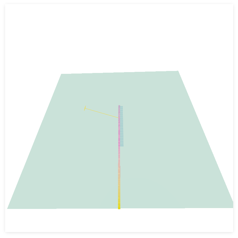
Next I created about 100 cubes as a first go at recreating the column of rectangles that are in the SVG version. However, when I saw the result I noticed that this pillar was getting much too long. To be able to see it fully the camera would have to be so far away that you couldn’t really appreciate the cubes and 3D aspect.
There was also something weird going on with the shadows not being visible for all cubes, but I tackled the position issue first.
I wanted to “fold” the long string of cubes into a 2D plane so it would take up less space. I therefore searched for how to create a Hilbert Curve with JavaScript. Thankfully, there exists a nifty hilbert-curve package that returns the position in the grid when you give it the index using hilbertCurve.indexToPoint(index, order)
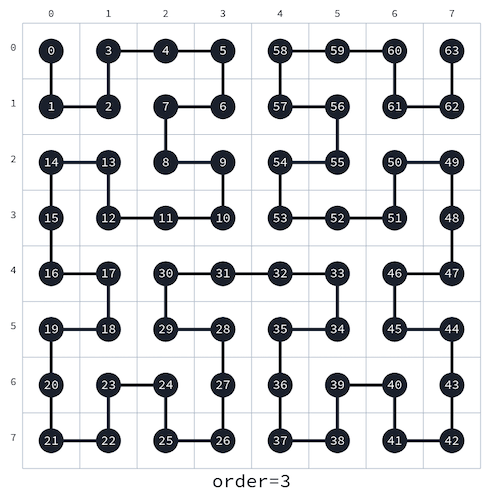
A size of the grid that forms a Hilbert curve goes in powers of two (the order). The phototransistor’s values range to a maximum value of 2^10 = 1024. Therefore, using a grid of 2^5 * 2^5 = 32 * 32 = 1024 was a perfect fit!
I placed 1024 cubes in the Hilbert grid layout, changed the position of the directional light to the bottom-left corner and noticed how the shadows were still clipped off quite oddly.
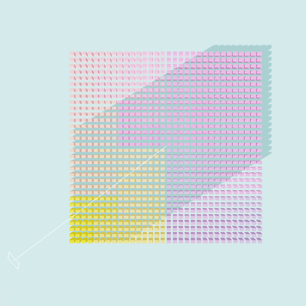
A few online searches later, and I understood that the frustum of the directional light wasn’t that big by default. However, I could increase it’s size and resolution by adding the settings from this forum post.
With the shadows fixed I connected the value that the phototransistor returns to which cubes are positioned above the ground plane (or below) at any point in time by checking if the index of a cube is greater or lower than the phototransistor’s value:
function animate() {
    if(serial_data) {
        //Possibly change the z-position of each cube
        meshes.forEach((mesh,i) => {
            if(i < serial_data) mesh.position.z = -scale/2
            else mesh.position.z = -scale*1.6
        })//forEach
    }//if
//// rest of animation function
}
This made the cubes appear and disappear suddenly:
To make this Three.js visual fit the style of the SVG and canvas version more, I made the ground plane update in color with the phototransistor’s value. I also wondered if I could add 3D text floating above the plane of cubes, since the previous visuals have a central text as well.
I found that there is a THREE.TextGeometry. However, you need to load a .json file that contains the outlines of the text (I think?).
Thankfully, there is Facetype.js which can convert any .ttf or .otf file into the required .json (even better, you can restrict the character set; I only needed the 10 number characters). From Google Fonts I downloaded Source Code Pro which I’ve been using in the other examples, and used Facetype.js to convert the Black font weight into a .json that I added to my project folder.
I used this example to get the TextGeometry actually working in my scene. The default TextGeometry settings I got from the Three.js website resulted in very blown-up text when I made the font size smaller (it says “123”):
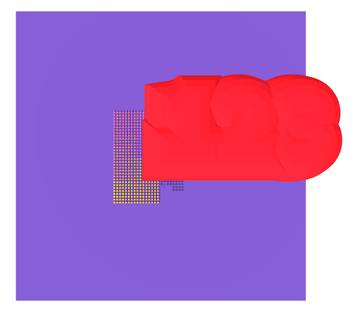
Some tweaking of the bevel settings later, and I had a huge white, but readable, text floating above my cubes.
There is no method to update the text of the geometry. Instead you have to remove the mesh from the scene, create one for the new text and add it. This is sadly heavy on the CPU. However, I also noticed that every new mesh I created for the value that came in from the serial connection, added to the memory being used by FireFox. At one point I got a warning from my Mac that the computer would crash soon because too much memory was being taken up, which came from FireFox using 61GB! (⑉⊙ȏ⊙)

I tried to find proper ways of disposing of meshes, and found this FAQ from Three.js. Using the two examples the FAQ share at the end I managed to severely reduce the amount of memory that FireFox grew with each second. I guess I couldn’t completely remove the increase in memory, but it was manageable now.
The final thing I wanted to tackle was the animation of the cubes. Right now they simple appeared or disappeared. I figured that using lerp (linear interpolation) between the current position of the cube and the position it should move to would give a nice animation.
While searching fow how to add lerp to Three.js I found that this is already part of the library, very handy! I followed this example to see the lerp() function used in an actual demo.
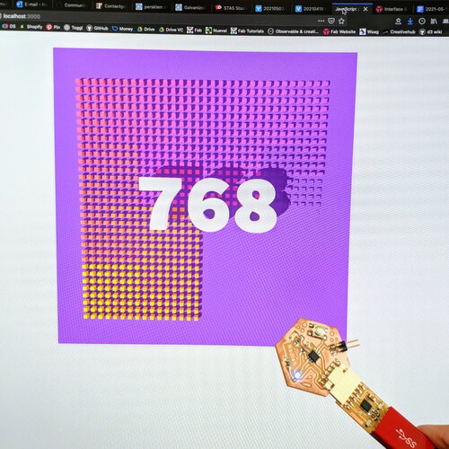
With that I had my Three.js visualization of the phototransistor’s value where I wanted it:
And below a photo where you can see the tiny board with the phototransistor that I’m getting my values from:
I have to admit, creating something this “silly” with Three.js was rather fun. I know that it doesn’t get really hard until you start writing your own vertex and fragment shaders (which is a whole rabbit hole of its own), but I’m happy with the result (^ᗨ^)
Below you can find the full folder with all the JavaScript and HTML files required to run the above example. As before, I’ve removed the node_modules folder because it’s insanely big, and you can install the required node modules running npm install (without any dependencies) in the terminal when you’re in the folder.
- Three.js visual files | ZIP file
P5.js
P5.js grew out of Processing and is basically Processing on the web, with JavaScript. It’s used by many artists, and is generally regarded as a very beginner friendly way to code. Many functions are very descriptive; want to draw a circle, use circle(), want to have a random number, use random(). I believe it’s a wrapper around HTML5 canvas actually.
I’ve only ever used p5.js during a 2-hour introduction workshop about two years ago. Although easy to use, I got the sense that I’d be able to all the things I could do with p5.js with D3.js as well, plus more, I therefore never investigated p5.js any deeper.
However, the predecessor to p5.js, Processing, is widely used by artists that create physical installations. I therefore expected that there might be an easy way for p5.js to work with “external” data, such as one coming from my board.
A quick online search on “Arduino p5.js” lead me to a tutorial that mentions the p5.serialport package (this tutorial, and this one also mention it).
I could’ve continued using the serialport way as I’ve been using up till now, together with the socket.io and express packages to get my data in the browser. However, the p5.serialport package actually seemed like it basically combined all those into one. With that I kind of mean, it literally combines them. Checking out the package.json I see that it uses both serialport and ws, the latter of which is an alternate package to socket.io.
I installed a global version of the package using npm install -g p5.serialserver, so I could use it everywhere, not just in the folder that I’d install it with using npm install.
By running p5serial in my terminal a web server is started, although I still need to configure the connection to the FTDI. I took the basic example code from the p5serial page and made some adjustments, such as inputting my FTDI id:
let serial
let data

const width = 400
const height = 400

function setup() {
    // Instantiate our SerialPort object
    serial = new p5.SerialPort()
    // Open the connection to my FTDI ID
    serial.open("/dev/tty.usbserial-D30A3T7C")

    /////// Register some callbacks ///////
    // When we connect to the underlying server
    serial.on('connected', () => { console.log("We are connected!") })
    // When we get a list of serial ports that are available

    // When or if we get an error
    serial.on('error', (err) => { console.log(err) })
    // When our serial port is opened and ready for read/write
    serial.on('open', () => { console.log("Serial Port is open!") })
    // When we some data from the serial port
    serial.on('data', gotData)

    /////////// Setup general p5.js stuff ///////////
    createCanvas(width, height)
}//function setup

function draw() {
    background('rgba(255,255,255, 0.1)')
    if (data) {
        document.getElementById("text-value").innerHTML = data
        circle(map(data, 0, 1023, 0, width), height/2, 80)
    }//if
}//function draw

// There is data available to work with from the serial port
function gotData() {
    let inString = serial.readLine();
    if (inString.length > 0) {
        data = Number(inString) //Convert it to a number
    }//if
}//function gotData
This resulted in the following messages in my terminal:
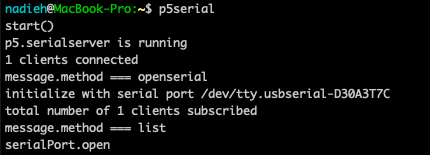
Interestingly, p5.js has a very similar setup as the Arduino IDE; there is a setup function that is called once when a page is loaded, and a draw function that is called continuously.
The example also mentions that I should add <script language="javascript" type="text/javascript" src="p5.serialport.js"> to the head of my index.html, which is the code for the client-side portion of the package.
I added a silly simple circle to the draw loop whose x-position is scaled to the value that the phototransistor returns: circle(map(data, 0, 1023, 0, width), height/2, 80). Thankfully that was all that was needed to setup the connection and get the phototransistor’s value in a browser. That was definitely easier that having to write you own server code as I did before.
Now that I had that working, I thought about what I find to be the “unique selling point” of p5.js. Since i’s basically canvas there is a big overlap. However, one of the things that define the coolness of p5.js to me is their noise function. The fact that they have Perlin noise integrated into their base program.
Basically, Perlin noise is a way to create nice looking randomness, instead of the normal chaos of randomness.
I own the book Generative Design, which teaches you about creating really amazing generative art with Processing. There’s also an updated version that switched to p5.js. Even better is that the book has a website where you can see all the code examples. From there I started from the M_1_5_03 example that really shows off the beauty of using Perlin noise.
I first made sure to get the code working on my localhost. Once I had, I looked through each line and added comments, making sure that I understood what was happening in each line.
Staying in style with my previous visuals, I wanted to update the look of each “agent” depending on the value that is measured from the phototransistor; using colors, opacities, stroke width and such.
The rest became just a whole lot of tweaking numbers, colors (using the tinyColor library to get a little more random colors around a main color), etc. and looking how the result appeared in my browser. I decided that it looked the best if I didn’t clear the background, but have each new loop of the draw() function to draw directly on what came before.
Once I had something that I liked, I wanted to add the central text. I used this reference from p5.js to load the text into my canvas. However, I then realized that I didn’t like the look, because you saw the numbers from all the previous draw() loops.

I therefore decoupled the text from the p5.s canvas. I placed the canvas that p5.js created in a specific <div>, that I gave and id of chart.
let canvas = createCanvas(width, height)
canvas.parent("chart")
I also added a <h1> to that <div> and turned that <div> into a CSS-grid. This makes it quite easy to horizontally and vertically overlap two HTML elements.
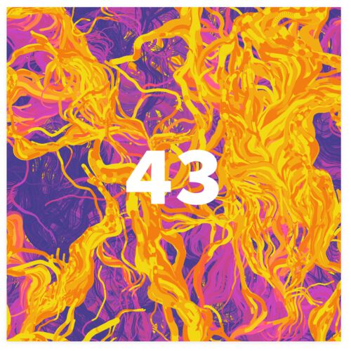
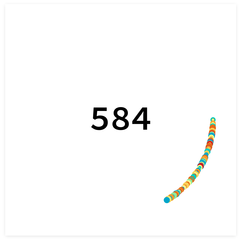
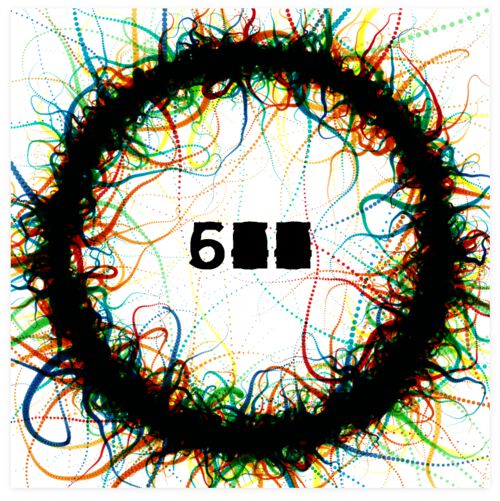
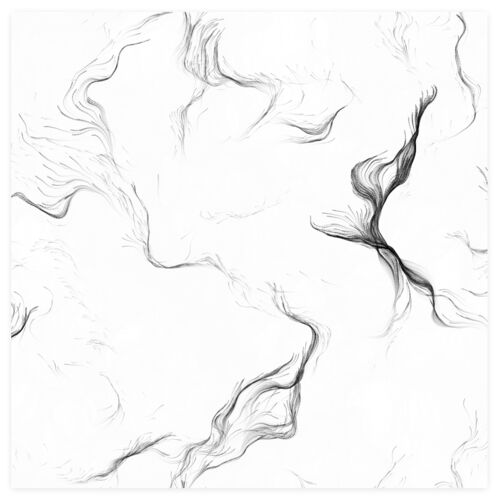
With that, my little example using p5.js was finished:
I like how the visual will never be the same, from second to the next. Even if the phototransistor shows the same number a few seconds later, the visual is already looking quite different in the meantime.

Below you can find the full folder with all the JavaScript and HTML files required to run the above example. Just to note, but you need to run p5serial before this example will work in the browser
- p5.js visual files | ZIP file
Serial with Data Analysis Tools
Besides the web, it might be handy to see if I can get a serial connection working with the two tools that I use for data preparation; R and python (although I use R in 95% of the cases and only use python if something isn’t possible in R).
R
For data preparation I prefer to work with R (using RStudio as the GUI). A quick online search showed that there is a serial package for R.
I installed the package and tried to run the example, changing the port to my FTDI and the baud rate to 9600:
library(serial)

con <- serialConnection(
  name = "FTDI",
  port = "tty.usbserial-D30A3T7C",
  mode = "9600,n,8,1", #<BAUD>,<PARITY>,<DATABITS>,<STOPBITS>
  newline = 1 #1 = transmission ends with newline
)
# let's open the serial interface
open(con)
# read, in case something came in
read.serialConnection(con)
# close the connection
close(con)
However, I never got the connection to successfully open. RStudio would just hang after running open(con). I’ve tried using different settings, and trying other options for the serialConnection function, but nothing worked.
One of my frustrations with R is that it’s bloody hard to google for. They should’ve used a name with more letters (ᗒᗣᗕ)՞ In this case I only found results about serial ports in general, often in combination with either Arduino or python. I did find three things for R, but these were not relevant to my problem, and thus couldn’t help me.
Perhaps I have the parity, databits, or stopbits wrong? But n,8,1 was what I saw in the few online examples that I could find…
Python
For python there is the pySerial package. I tried installing it with pip3 install pyserial, but it was apparently already installed (I think during the “Electronics Design” week).
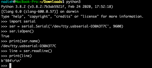
I used this example to get my own code going:
import serial
ser = serial.Serial(
    port = '/dev/tty.usbserial-D30A3T7C',\
    baudrate = 9600)
ser.flushInput()
#print(ser.isOpen())

while True:
    try:
        line = ser.readline()
        try:
            line_decoded = int(line.decode("utf-8"))
            print(line_decoded)
        except:
            continue
    except:
        break
It seems that (for me at least), running the serial.Serial also immediately opens the connections (you can check with ser.isOpen()).
Running the ser.readline() gives the number from the phototransistor. It does still need to be decoded using .decode("utf-8"), otherwise you get results such as b'984\r\n' .
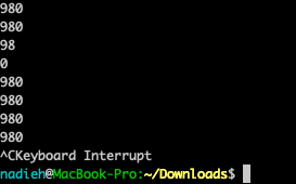
I think I noticed that running ser.readline() for the second time gives the second value that the phototransistor ever send, not the value send at that moment by my board (or perhaps it’s the second value in the buffer?). I therefore used the while loop to make sure that the latest value is always taken/printed.
I also had to add another try because the while loop tries to query the serial line more often than every 100 milliseconds (which is how often my board sends it out). I therefore often got empty results back that crashed my program. The second try therefore checks if the returned result is an integer, and if yes, prints it to my terminal.
At first I had a timeout=0 added to the serial.Serial statement, but it resulted in sometimes the value from the phototransistor being cut in two separate numbers, such as first 98 and then 0. Removing the timeout fixed that issue.
I also had an error for a while because I’d named my own file serial.py, which made the import serial statement fail. I adjusted the name of my file to something else and then it worked again.
Knowing that I could set-up the serial connection within python and receive the values (as integers/numbers) was enough for me. I never use python (or R) to create visualizations to show to anybody else. I only use it for myself during the data cleaning and analysis phase, as a quick understanding of what’s in the data. I therefore figured I could spend my time more wisely on my final project, than visualizing the incoming number through a chart in python.
Group Assignment
During the local class, I explained the main strengths and differences of using D3.js, HTML5 canvas and Three.js, showing some examples that I’ve made in the past. I then helped the rest of the group through a tutorial to get a local host working on their Mac. I felt that having a local host working would/might become really handy for some of them later this week, or when they need JavaScript for their final project.
The next Monday I gave a Zoom presentation to our regional group in which I build up an “exotic” data visualization (about the number of babies born per day in the US) using D3.js, just to give those interested what it’s like to work with D3.js, because I felt it would be too difficult to pick up well in just one week.
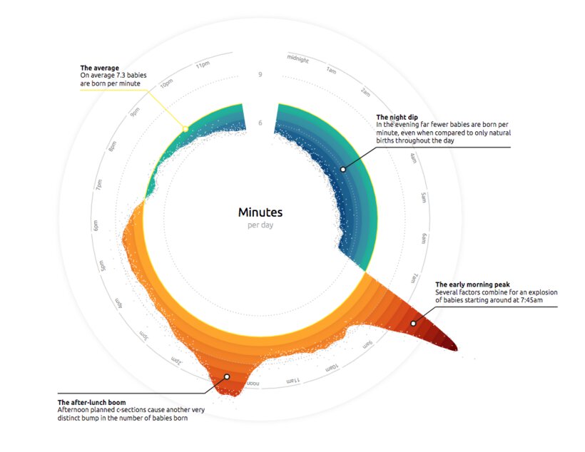
Here is a recording of the presentation. But be warned, this is not an introduction to D3.js. I’m trying to show the capabilities of D3.js, and to show the process of creating a custom data visualization through code. So if you’re interested, I’d advice you to just sit back and take it in without trying to understand every line of code I’m typing.
Reflections
This was a fun week! Probably not so unexpected, since I make the visualization of data my job. Nevertheless, it was fun getting to play with all of these different JavaScript based tools within one week, and trying to think about how to use the strengths and unique selling points of each tool.
It was also half a week, because the second half of the week I focused on my final project, working on the bottom plate of my puzzle.
What went wrong
Thankfully, nothing big went wrong this week. However, I wish I’d been able to set up the serial connection to R, since this is a program that I almost always use to prepare and analyze my data.
What went well
I managed to finish the examples for D3.js, HTML5 canvas, Three.js and p5.js within an hour or 2-3 for each, and I like how they all came together and I managed to get the same visual style working in all of them (^▽^)
What I would do differently
If the Web Serial API ever gets supported by more browsers than Chrome and Edge (I’d need at least FireFox and preferably also Safari), I’d be interested in trying it. But until that point arrives, I’ll leave it.
Wrapping up
Because I work with user interfaces and visualizing on the web for my job, I intentionally didn’t add any kind of display for my final project. Doing UI well, including taking resizing / any screen width into account, browser performance and browser bugs, takes about 80% of any of my projects. Here I did the most fun 20% part of the process. I know that for my final project I’d want to do it properly if I had a display, and thus the best solution to keep things as fun as possible was to have no display at all. I also don’t know what I would really need a display for with my puzzle anyway. Or in short, this was a fun week, I’m very happy I learned how to connect to a serial port, but I’ll not need it specifically for my final project (^.~)